Reading Report – Management of Disasters #6

Book Name:

Part 3 / Implementation of systems analysis to management of disasters: Chapter 6 / Optimization

Summary

The procedure of selecting the set of decision variables that maximizes or minimizes the objective function, subject to the systems constraints, is called the optimization procedure. Linear programming is applied to problems that are formulated in terms of separable objective functions and linear constraints. In order to formulate the mathematical model in terms of linear relationships, 4 conditions must be satisfied

• Proportionality: For each activity, the total amounts of each input and the associated value of the objective are strictly proportional to the level of output that is, to the activity level. Each activity is capable of continuous proportional expansion or reduction.
• Additivity: Given the activity levels for each of the decision variables xj, the total amounts of each input and the associated value of the objective are the sums of the inputs and objective values for each individual process.
• Divisibility: Activity units can be divided into any fractional levels so that non-integer values for the decision variables are permissible.
• Certainty: All the parameters of the linear model are known constants.

The first step is to decide which are the decision variables. These are the quantities that can be varied, and so affect the value of the objective. The second step in the formulation is to express the objective in terms of the decision variables. Lastly, we must write down the constraints that restrict the choices of decision variables. Letting xj be the level of activity j, for j = 1, 2, . . . , n, we want to select a value for each xj such that:

C1x1 + C2x2 +· · ·+Cn xn

is maximized or minimized, depending on the context of the problem. The xj are constrained by a number of relations, each of which is one of the following type:

a1x1 + a2x2 +· · ·+an xn ≤ a

b1x1 + b2x2 +· · ·+bn xn = b

c1 x1 + c2x2 +· · ·+cn xn ≥ c

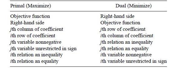
Whenever an LP model is formulated and solved, the result will be one of four characteristic solution types shown in figure 6.2.

1. Unique Optimal Solution: The point (6, 4) in figure 6.1(a) is the only point that satisfied all constraint equations simultaneously. Consequently, the optimal solution to the linear program is a unique one; the solution is said to have a unique optima
2. Alternate optimal solutions: the orientation of the objective function in decision space is determined by the coefficient that multiply the decision variables. For example, if the coefficient on x2 in the original objective function is decreased relative to the coefficient on x1, the gradient becomes steeper. This problem thus has an infinite number of optimal solutions, or is said to have alternate optima. Alternate optima are actually more common as the size of the LP problem increases, and it is important to be able to recognize their presence.
3. Infeasible solution: It is possible that there are no feasible solutions for a given problem formulation, or due to errors in formulating logical constraints or mistakes in inputting a problem formulation to a model solver, the problem is over-constrained to the extent that there is no solution satisfying all constraint equations simultaneously
4. Unbounded solution : As infeasible problems result from problems that are over-constrained, we may also encounter problems that are under-constrained. The feasible region is shown shaded and constrained by three constraints. The objective function gradient and its direction of improvement are also shown. Note that for any feasible solution in this decision space, we can always find another solution that gives a better value of the objective function such that the objective function for this problem could be moved upward and to the right without limit. Such a problem is said to be unbounded

Many different algorithms have been proposed to solve LP problems, but the one below has proved to be the most effective in general. This is the general procedure:

Step 1: Select a set of m variables that yields a feasible starting trial solution. Eliminate the selected m variables from the objective function.

Step 2: Check the objective function to see whether there is a variable that is equal to 0 in the trial solution but would improve the objective function if made positive. If such a variable exists, go to step 3. Otherwise, stop.

Step 3: Determine how large the variable found in the previous step can be made until one of the m variables in the trial solution becomes 0. Eliminate the latter variable and let the next trial set contain the newly found variable instead.

Step 4: Solve for these m variables, and set the remaining variables equal to 0 in the next trial solution. Return to step 2.

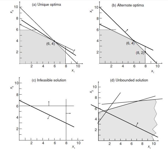
Figure 6.1 Linear program solutions: (a) unique optimal solution, (b) alternate optimal solution, (c) infeasible solution, and (d) unbounded optimal solution.

Sensitivity analysis is the study of how the optimal solution and the value of the optimal solution to a linear program change, given changes in the various coefficient of the problem. The author introduced 3 types of the sensitivity analysis which are the coefficient of the objective function, the right-hand sides and the matrix of the left-hand side coefficient. Duality establishes the interconnections for all of the sensitivity analysis techniques. We arbitrarily call (Eq. 6.1) the primal problem and (Eq. 6.2) its dual problem. The dual problem can be viewed as the primal model flipped on its side. The duality relationships are summarized in Table 6.1.

(Eq.6.1)

(Eq.6,2)

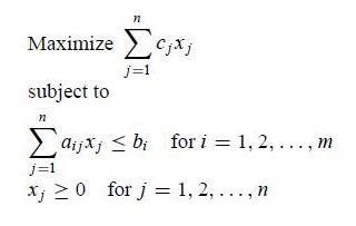
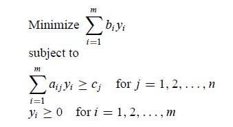
Table 6.1 Relationship between Primal and Dual Problems

The transportation problem is a special type of LP problem, The special procedure used to solve the transportation LP problem is known as the transportation simplex method. The general transportation problem is concerned with distributing any commodity from any group of supply centers sources, to any group of receiving centers, called destinations, in such a way as to minimize the total distribution cost. A basic assumption is that the cost of distributing units from source i to destination j is directly proportional to the number distributed, where cj denotes the cost per unit distributed. Letting Z be total distribution cost and xij (i = 1, 2,…, m; j = 1, 2,…, n) be the number of units to be distributed from source i to destination j, the LP formulation of this problem becomes:

A necessary and sufficient condition for a transportation problem to have any feasible solutions is that  .

The condition that the total supply must equal the total demand merely requires that the system be in balance. To demonstrate the modified solution method for the transportation problem, the author used a transportation simplex tableau shown in Figure 6.2

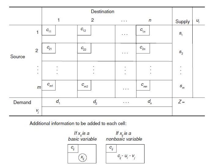
Figure 6.2 Format of transportation simplex tableau.

Implementation of the transportation simplex method proceeds as follows:

1. Initialization step: Construct an initial basic feasible solution. Go to the optimality test.

2. Iterative step:

– Determine the entering basic variable. Select the non-basic variable xij having the largest (in absolute terms) negative value of ( cij−ui−vj ).  —– Determine the leaving basic variable. Identify the chain reaction required to retain feasibility when the entering basic variable is increased. From among the donor cells, select the basic variable having the smallest value.

– Determine the new basic feasible solution. Add the value of the leaving basic variable to the allocation for each recipient cell. Subtract this value from the allocation for each donor cell.

3. Optimality test: Derive the ui and vj by selecting the row having the largest number of allocations and setting its ui =0 and then solving the set of equations cij = ui + vj for each (i, j) such that xij is basic. If (cij − ui − vj) ≥ 0 for every (i, j) such that xij is non-basic, then the current solution is optimal, so stop. Otherwise, go back to step 2.

Network representations are widely used in distribution, project planning, facilities location resource management, and financial planning. A network representation provides the most powerful visual and conceptual aid for describing the relationships between the components of systems. A network consists of a set of points and a set of lines connecting certain pairs of the points which are called nodes. The lines are called arcs. Arcs are labeled by naming the nodes at either end; AB is the arc between nodes A and B. The arcs of a network may have a flow of some type through them. If flow through an arc is allowed only in one direction, the arc is said to be a directed arc. If the flow through an arc is allowed in both directions, the arc is said to be an undirected arc. A network that has only directed arcs is called a directed network. If all of its arcs are undirected, the network is said to be an undirected network. A network with a mixture of directed and undirected arcs can be converted into a directed network by replacing each undirected arc by a pair of directed arcs in opposite directions. When two nodes are not connected by an arc, they may be connected by a path that is define as a sequence of distinct arcs connecting these nodes. When some or all of the arcs in the network are directed arcs, we then distinguish between directed paths and undirected paths. A directed path from node i to node j is a sequence of connecting arcs whose direction is toward node j, so that flow from node I to node j along this path is feasible. An undirected path from node i to node j is a sequence of connecting arcs whose direction can be either toward or away from node j. To illustrate these definitions Figure 6.3 shows a typical directed network.

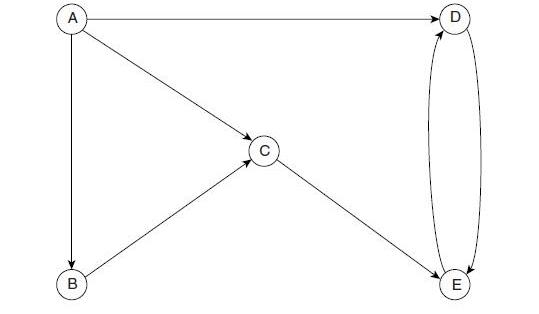
Figure 6.3 Example of a directed network.

Reporter’s Own Thoughts

I think the optimization method is one of the methods that have so many tools for the analyst to choose them according to the specific type of problem they trying to solve. I summarize the basic and some procedure of the tools but did not include the example which will make the explanation easier to understand but if you are interesting the example from the book is quite interesting.